线性回归模型

线性回归模型

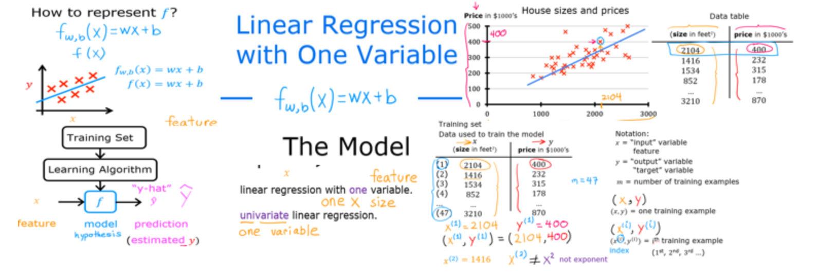
MOdel Representation

Goals

In this lab you will:

• learn to implement the model f_{w,b} for linear regression with one variable

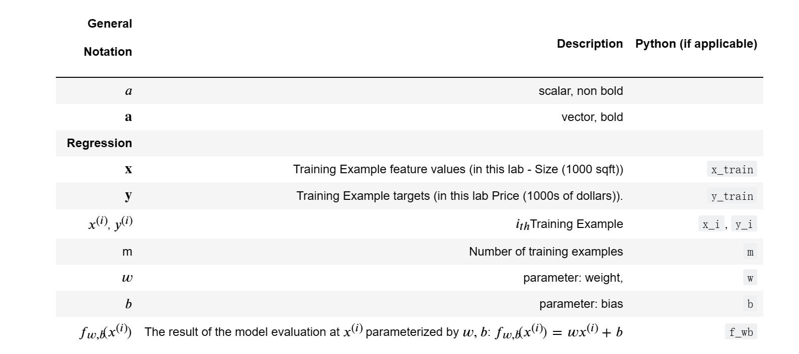
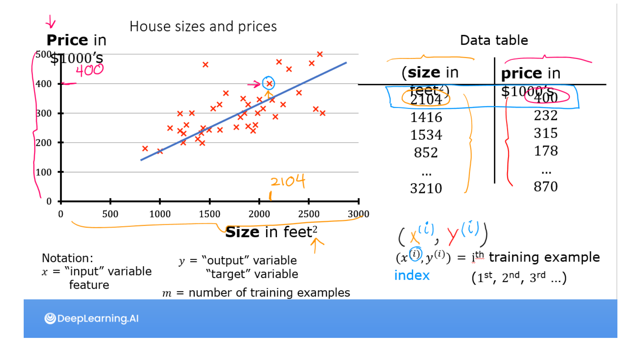
Notation

Here is a summary of some of the notation you will encounter.

Tools

In this lab you will make use of:

• NumPy,a popular library for scientific computing

• Matplotlib,a popular library for plotting data

  import numpy as np
  import matplotlib.pyplot as plt
  plt.style.use('./deeplearning.mpstyle')

Problem Statement

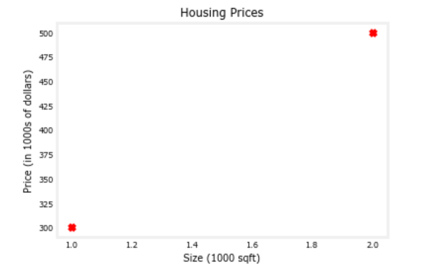
As in the lecture,you will use the motivating example of housing price prediction. This lab will use a simple data set with only two data points - a house with 1000 square feet(sqft) sold for $300,000 and a house with 2000 square feet sold for $500,000.These two points will constitute our data or training set. In this lab, the units of size are 1000 sqft and the units of price are 1000s of dollars.

Size (1000 sqft)	Price (1000s of dollars)
1.0	300
2.0	500

You would like to fit a linear regression model(shown above as the blue straight line)through these two points, so you can then predict price for other houses - say, a house with 1200 sqft.

Please run the following code cell to create your x_train and y_train variables. The data is stored in one-dimensional NumPy arrays.

#x_train is the input variable (size in 1000 square feet)
#y_train is the target (price in 1000s of dollars)
x_train = np.array([1.0,2.0])
y_train = np.array([300.0,500.0])
print(f"x_train = {x_train}")
print(f"y_train = {y_train}")

Number of training examples m

you will use m to denote the number of training examples. Numpy arrays have a .shape parameter. x_train.shape return a python tuple with an entry for each dimension. x_train.shape[0] is the length of the array and number of examples as shown below.

# m is the number of training examples
print(f"x_train.shape: {x_train.shape}")
m = x_train.shape[0]
print(f"Number of training example is: {m}")

x.train.shape: (2,)

Number of training examples is: 2

One can also use the Python len() function as shown below.

# m is the number of training examples
m = len(x_train)
print(f"Number of training example is: {m}")

Number of training examples is: 2

Training example x_i, y_i

You will use (x(𝑖), y(𝑖)) to denote the 𝑖(th) training example. Since Python is zero indexed, (x(0), y(0) is (1.0, 300.0) and (x(1), y(1) is (2.0, 500.0).

To access a value in a Numpy array, one indexes the array with the desired offset. For example the syntax to access location zero of x_train is x_train[0]. Run the next code block below to get the i(th) training example.

i = 0 #Change this to 1 to see (x^1,y^1)

x_i = x_train[i]
y_i = y_train[i]
print(f"(x^({i}), y^({i})) = ({x_i}, {y_i})")

(x^(0), y^(0)) = (1.0, 300.0)

Plotting the data

You can plot these two points using the scatter() function is the matplotlib library,as shown in the cell below.

• The function arguments marker and c show the points as red crosses(the default is blue dots.)

You can use other functions in the matplotlib library to set title and labels to display.

#Plot the data points
plt.scatter(x_train, y_train, marker='x' c='r')
#Set the title
plt.title("Housing Prices")
#Set the y-axis label
plt.ylabel('Price (in 1000s of dollars)')
#Set the x-axis lbel
plt.xlabel('Size (1000 sqft)')
plt.show()

Model function

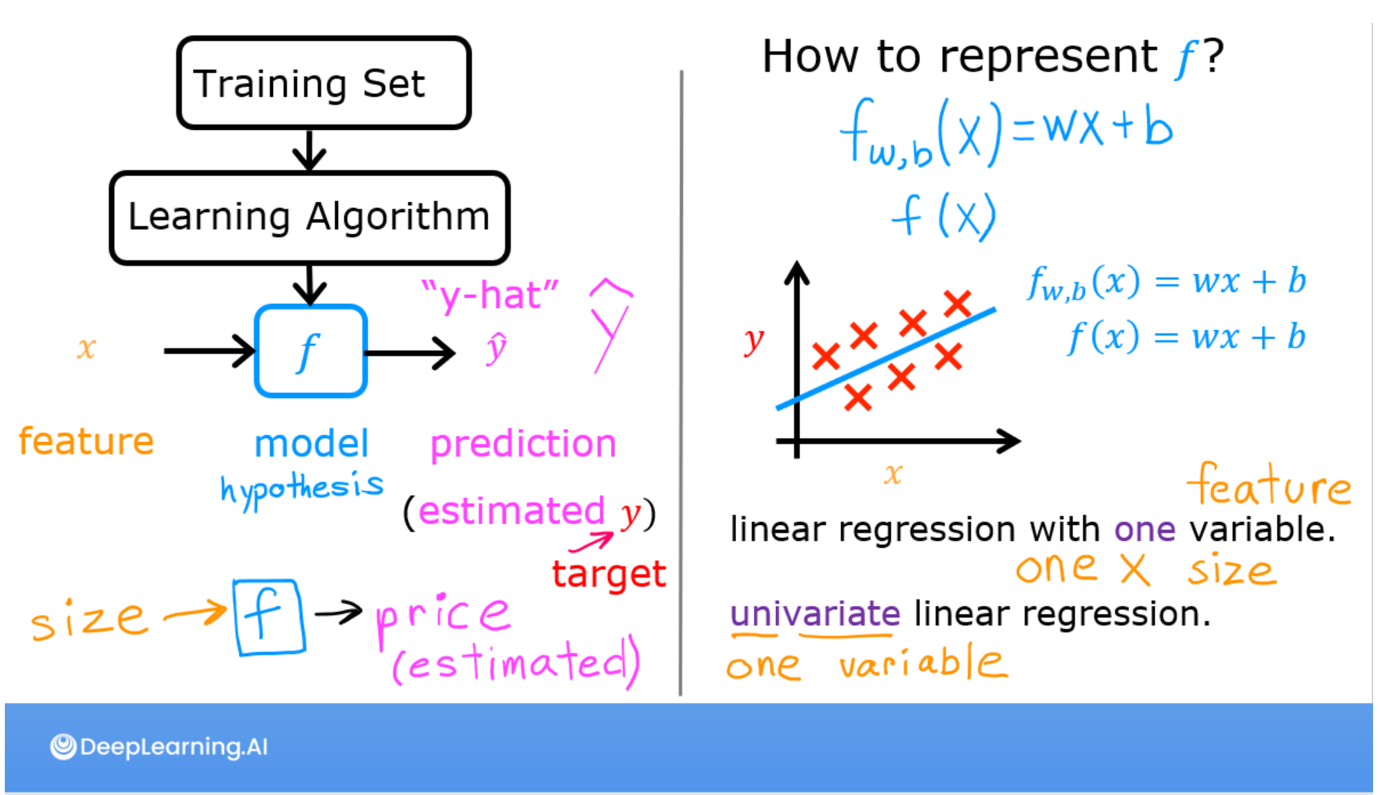
As described in lecture, the model function for linear regression (which is a function that maps from x to y)is represented as

The formula above is how you can represent straight lines - different values of w and b give you different straight lines on the plot.

Let’s try to get a better intuition for this through the code blocks below. Let’s start with w = 100 and b =100.

Note: You can come back to this cell to adjust the model’s w and b parameters.

w = 100
b = 100
print(f"w: {w}")
print(f"b: {b}")

w:	100
b:	100

Now,let’s compute the value of f_{w,b}(x^i) for your two data points. You can explicitly write this out for each data poins as -

for x(0),f_wb = w * x[0] + b

for x(1),f_wb = w * x[1] + b

For a large number of data points, this can get unwieldy and repetitive. So instead, you can calculate the function output in a for loop as shown in the compute_model_output function below.

Note:The argument description (ndarray (m,)) describes a Numpy n-dimensional array of shape (m,). (scalar) describes an argument without dimensions, just a magnitude.

Note: np.zero(n) will return a one-dimensional numpy array with n entries

def compute_model_output(x, w, b):
    """
    Computes the prediction of a linear model
    Args:
    	x (ndarray (m,)):Data, m examples
    	w,b (scalar)	:model parameters
    Returns
    	y (ndarray (m,)):target values
    """
    
    m = x.shape[0]
    f_wb = np.zeros(m)
    for i in range(m)
    	f_wb[i] = w * x[i] + b
    
    return f_wb

Now let’s call the compute_model_output function and plot the output.

tmp_f_wb = compute_model_output(x_train, w, b,)

#Plot our model prediction
plt.plot(x_train, tmp_f_wb, c='b',label='Our Prediction')

#Plot the data points
plt.scatter(x_train, y_train, marker='x', c='r',label='Actual Values')

#Set the title
plt.title("Housing Prices")
#Set the y-axis label
plt.ylabel('Price (in 1000s of dollars)')
#Set the x-axis label
plt.xlabel('Size (1000 sqft)')
plt.legend()
plt.show()

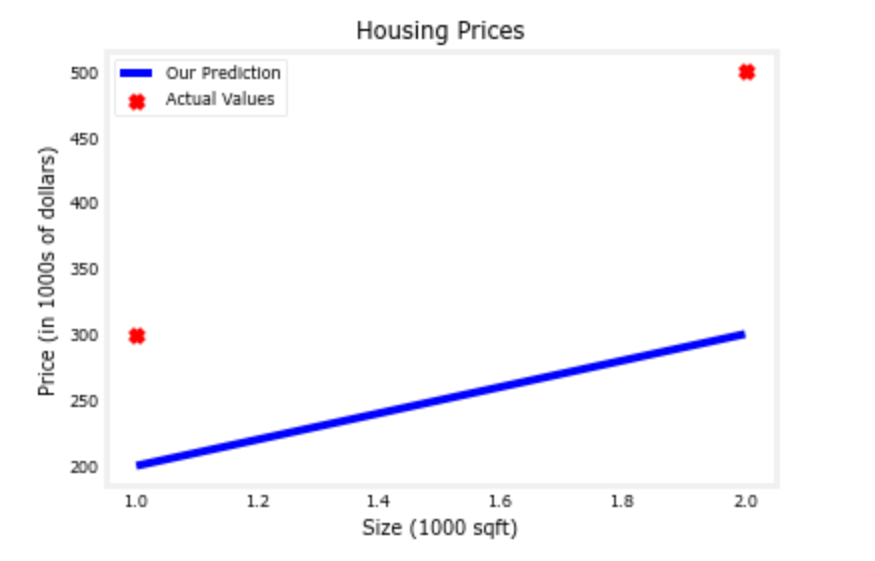
As you can see, setting w = 100 and b = 100 does not result in a line that fits our data.

Challenge

Try experimenting with different values of w and b. What should the values be for a line that fits our data?

Tips:

You can use your mouse to click on the triangle to the left of the green “Hints” below to reveal some hints for choosing b and w.

Hints

Prediction

Now that we have a model, we can use it to make our original prediction. Let’s predict the price of a house with 1200 sqft. Since the units of x are in 1000’s of sqft, x is 1.2.

w = 200
b = 100
x_i = 1.2
cost_1200sqft = w * x_i + b
print(f"${cost_1200sqft:.0f} thousand dollars" )

$340 thousand dollars

Congratulations!

In this lab you have learned:

• Linear regression bulids a model which establishes a relationship between features and targets
• In the example above, the feature was house size and the target was house price
• for simple linear regression, the model has two parameters w and b whose calue are ‘fit’ using training data.
• once a model’s parameters have been determined, the model can be used to make predictions on novel data.

参考资料

https://www.bilibili.com/video/BV1Pa411X76s?p=5&vd_source=3ae32e36058f58c5b85935fca9b77797

kaieye/2022-Machine-Learning-Specialization (github.com)