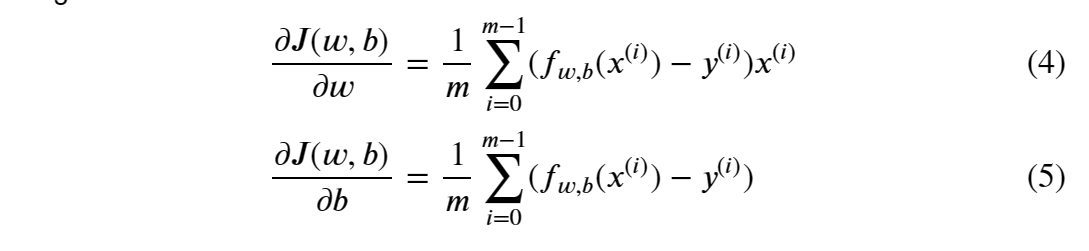
线性回归的梯度下降

线性回归的梯度下降

image-20230313145346118

Goals

在本实验中,您将:

  • 使用梯度下降自动优化w和b的过程

Tools

在本实验中,我们将使用:

  • NumPy,一个用于科学计算的流行库
  • Matplotlib,用于绘制数据的流行库
  • 在本地目录的lab_utils.py文件中绘制例程
1
2
3
4
5
import math, copy
import numpy as np
import matplotlib.pyplot as plt
plt.style.use('./deeplearning.mplstyle')
from lab_utils_uni import plt_house_x, plt_contour_wgrad, plt_divergence, plt_gradients

Problem Statement

让我们使用与之前相同的两个数据点——1000平方英尺的房子以30万美元的价格出售,2000平方英尺的房子以50万美元的价格出售。

Size(1000 sqft)Price(1000s of dollars)
1300
2500
1
2
3
#Load our data set
x_train = np.array([1.0, 2.0]) #features
y_train = np.array([300.0,500.0]) #target value

Compute_Cost

这是上一个实验室开发的。我们在这里还会用到它。

1
2
3
4
5
6
7
8
9
10
11
12
#Function to calculate the cost
def compute_cost(x, y, w, b,):

m = x.shape[0]
cost = 0

for i in range(m):
f_wb = w * x[i] + b
cost = cost + (f_wb - y[i])**2
total_cost = 1 / (2 * m)*cost

return total_cost

Gradient descent summary

到目前为止,在这门课程中,你已经建立了一个线性模型来预测f_w,b(x^i):

image-20230313150848463

在线性回归中,您使用输入训练数据来拟合参数𝑤,𝑏;来最小化我们的预测之间的误差测量f_𝑤,𝑏(𝑥^(𝑖))和实际数据𝑦(𝑖)。这种测量成为代价,J(w,b)。在训练中,你可以衡量我们所有训练样本的成本𝑥(𝑖),𝑦(𝑖)。

image-20230313151251919

在课堂上,梯度下降被描述为:

image-20230313151329621

其中参数𝑤,𝑏同时更新。

image-20230313151450500

这里同时意味着在更新任何参数之前计算所有参数的偏导数。

Implement Gradient Descent

你将为一个特征实现梯度下降算法。你需要三个函数。

  • compute_gradient实现上述式(4)和(5)
  • 上面的compute_cost实现方程(2)(代码来自以前的实验室)
  • gradient_descent,使用compute_gradient和compute_cost

Conventions:

image-20230313151857315

compute_gradient

image-20230313151947363

1
2
3
4
5
6
7
8
9
10
11
12
13
14
15
16
17
18
19
20
21
22
23
24
25
26
27
def compute_gradient(x, y, w, b):
"""
Computes the gradient for linear regression
Args:
x (ndarray (m,)): Data, m examples
y (ndarray (m,)): target values
w,b (scalar) : model parameters
Returns
dj_dw (scalar): The gradient of the cost w.r.t. the parameters w
dj_db (scalar): The gradient of the cost w.r.t. the parameter b
"""

#Number of training examples
m = x.shape[0]
dj_de = 0
dj_db = 0

for i in range(m):
f_wb = w * x[i] + b;
dj_dw_i = (f_wb - y[i]) * x[i]
dj_db_i = f_wb - y[i]
dj_db += dj_db_i
dj_dw += dj_dw_i
dj_dw = dj_dw / m
dj_db = dj_db / m
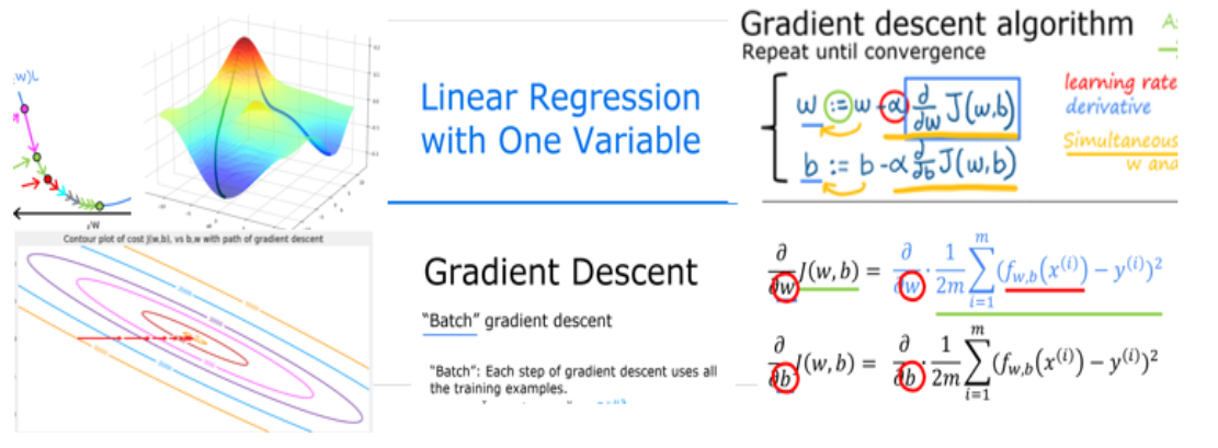
return dj_dw, dj_db

课程描述了梯度下降如何利用在某一点上对参数代价的偏导数来更新该参数。

让我们使用compute_gradient函数来查找并绘制代价函数相对于其中一个参数𝑤0的偏导数。

image-20230313154012173

1
2
plt_gradients(x_train,y_train, compute_cost, compute_gradient)
plt.show()

image-20230313154210478

image-20230313154333429

Gradient Descent

现在可以计算梯度,上面公式(3)中描述的梯度下降可以在下面的gradient_descent中实现。注释中描述了实现的细节。下面,您将利用这个函数在训练数据上找到w和b的最佳值。

1
2
3
4
5
6
7
8
9
10
11
12
13
14
15
16
17
18
19
20
21
22
23
24
25
26
27
28
29
30
31
32
33
34
35
36
37
38
39
40
41
42
43
44
45
46
47
def gradient_descent(x, y, w_in, b_in, alpha, num_iters, cost_function, gradient_function): 
"""
Performs gradient descent to fit w,b. Updates w,b by taking
num_iters gradient steps with learning rate alpha

Args:
x (ndarray (m,)) : Data, m examples
y (ndarray (m,)) : target values
w_in,b_in (scalar): initial values of model parameters
alpha (float): Learning rate
num_iters (int): number of iterations to run gradient descent
cost_function: function to call to produce cost
gradient_function: function to call to produce gradient

Returns:
w (scalar): Updated value of parameter after running gradient descent
b (scalar): Updated value of parameter after running gradient descent
J_history (List): History of cost values
p_history (list): History of parameters [w,b]
"""

w = copy.deepcopy(w_in) # avoid modifying global w_in
# An array to store cost J and w's at each iteration primarily for graphing later
J_history = []
p_history = []
b = b_in
w = w_in
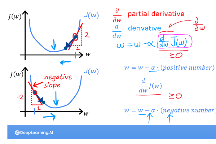
for i in range(num_iters):
# Calculate the gradient and update the parameters using gradient_function
dj_dw, dj_db = gradient_function(x, y, w , b)

# Update Parameters using equation (3) above
b = b - alpha * dj_db
w = w - alpha * dj_dw

# Save cost J at each iteration
if i<100000: # prevent resource exhaustion
J_history.append( cost_function(x, y, w , b))
p_history.append([w,b])
# Print cost every at intervals 10 times or as many iterations if < 10
if i% math.ceil(num_iters/10) == 0:
print(f"Iteration {i:4}: Cost {J_history[-1]:0.2e} ",
f"dj_dw: {dj_dw: 0.3e}, dj_db: {dj_db: 0.3e} ",
f"w: {w: 0.3e}, b:{b: 0.5e}")

return w, b, J_history, p_history #return w and J,w history for graphing
1
2
3
4
5
6
7
8
9
10
11
Iteration    0: Cost 7.93e+04  dj_dw: -6.500e+02, dj_db: -4.000e+02   w:  6.500e+00, b: 4.00000e+00
Iteration 1000: Cost 3.41e+00 dj_dw: -3.712e-01, dj_db: 6.007e-01 w: 1.949e+02, b: 1.08228e+02
Iteration 2000: Cost 7.93e-01 dj_dw: -1.789e-01, dj_db: 2.895e-01 w: 1.975e+02, b: 1.03966e+02
Iteration 3000: Cost 1.84e-01 dj_dw: -8.625e-02, dj_db: 1.396e-01 w: 1.988e+02, b: 1.01912e+02
Iteration 4000: Cost 4.28e-02 dj_dw: -4.158e-02, dj_db: 6.727e-02 w: 1.994e+02, b: 1.00922e+02
Iteration 5000: Cost 9.95e-03 dj_dw: -2.004e-02, dj_db: 3.243e-02 w: 1.997e+02, b: 1.00444e+02
Iteration 6000: Cost 2.31e-03 dj_dw: -9.660e-03, dj_db: 1.563e-02 w: 1.999e+02, b: 1.00214e+02
Iteration 7000: Cost 5.37e-04 dj_dw: -4.657e-03, dj_db: 7.535e-03 w: 1.999e+02, b: 1.00103e+02
Iteration 8000: Cost 1.25e-04 dj_dw: -2.245e-03, dj_db: 3.632e-03 w: 2.000e+02, b: 1.00050e+02
Iteration 9000: Cost 2.90e-05 dj_dw: -1.082e-03, dj_db: 1.751e-03 w: 2.000e+02, b: 1.00024e+02
(w,b) found by gradient descent: (199.9929,100.0116)

花点时间,注意上面打印的梯度下降过程的一些特征。

  • 正如课堂上的幻灯片所描述的,成本开始很大,然后迅速下降。
  • 偏导数dj_dw和dj_db也变小了,起初很快,然后变慢。正如课堂上的图表所示,随着过程接近“碗底”,由于在这一点上的导数值较小,进程会变慢。
  • 尽管学习率alpha保持不变,但进程会减慢

image-20230313155614815

Cost versus iterations of gradient descent

成本与迭代的关系图是衡量梯度下降技术进展的有用方法。在成功的运行中,成本总是会降低。最初成本的变化如此之快,用不同于最终下降的尺度来描绘最初的上升是有用的。

在下面的图表中,请注意轴上的成本规模和迭代步骤。

1
2
3
4
5
6
7
8
# plot cost versus iteration  
fig, (ax1, ax2) = plt.subplots(1, 2, constrained_layout=True, figsize=(12,4))
ax1.plot(J_hist[:100])
ax2.plot(1000 + np.arange(len(J_hist[1000:])), J_hist[1000:])
ax1.set_title("Cost vs. iteration(start)"); ax2.set_title("Cost vs. iteration (end)")
ax1.set_ylabel('Cost') ; ax2.set_ylabel('Cost')
ax1.set_xlabel('iteration step') ; ax2.set_xlabel('iteration step')
plt.show()

image-20230313160112122

Predictions

现在您已经发现了参数𝑤的最佳值和𝑏,您现在可以使用该模型根据我们学习的参数来预测房屋价值。正如预期的那样,在相同的住房条件下,预测值与训练值几乎相同。进一步,不在预测中的值与期望值一致。

1
2
3
print(f"1000 sqft house prediction {w_final*1.0 + b_final:0.1f} Thousand dollars")
print(f"1200 sqft house prediction {w_final*1.2 + b_final:0.1f} Thousand dollars")
print(f"2000 sqft house prediction {w_final*2.0 + b_final:0.1f} Thousand dollars")
1
2
3
1000 sqft house prediction 300.0 Thousand dollars
1200 sqft house prediction 340.0 Thousand dollars
2000 sqft house prediction 500.0 Thousand dollars

Plotting

您可以通过在代价(w,b)的等高线图上绘制迭代的代价来显示梯度下降在执行过程中的进度。

1
2
fig, ax = plt.subplots(1,1, figsize=(12, 6))
plt_contour_wgrad(x_train, y_train, p_hist, ax)

image-20230313160446994

上面的等高线图显示了𝑤和𝑏范围内的𝑐𝑜𝑠𝑡(𝑤,𝑏)。成本水平由圆环表示。用红色箭头覆盖的是梯度下降的路径。这里有一些需要注意的事情:

  • 这条路径朝着它的目标稳步(单调)前进。
  • 最初的步骤比接近目标的步骤要大得多。

放大,我们可以看到梯度下降的最后步骤。注意,阶梯之间的距离随着梯度趋近于零而缩小。

1
2
3
fig, ax = plt.subplots(1,1, figsize=(12, 4))
plt_contour_wgrad(x_train, y_train, p_hist, ax, w_range=[180, 220, 0.5], b_range=[80, 120, 0.5],
contours=[1,5,10,20],resolution=0.5)

image-20230313160944244

Increased Learning Rate

在这节课中,在式(3)中有一个关于学习率的合适值𝛼的讨论。𝛼越大,梯度下降收敛到解的速度就越快。但是,如果它太大,梯度下降就会发散。上面有一个很好收敛的解的例子。让我们试着增加𝛼的值看看会发生什么:

image-20230313161516209

1
2
3
4
5
6
7
8
9
# initialize parameters
w_init = 0
b_init = 0
# set alpha to a large value
iterations = 10
tmp_alpha = 8.0e-1
# run gradient descent
w_final, b_final, J_hist, p_hist = gradient_descent(x_train ,y_train, w_init, b_init, tmp_alpha,
iterations, compute_cost, compute_gradient)
1
2
3
4
5
6
7
8
9
10
Iteration    0: Cost 2.58e+05  dj_dw: -6.500e+02, dj_db: -4.000e+02   w:  5.200e+02, b: 3.20000e+02
Iteration 1: Cost 7.82e+05 dj_dw: 1.130e+03, dj_db: 7.000e+02 w: -3.840e+02, b:-2.40000e+02
Iteration 2: Cost 2.37e+06 dj_dw: -1.970e+03, dj_db: -1.216e+03 w: 1.192e+03, b: 7.32800e+02
Iteration 3: Cost 7.19e+06 dj_dw: 3.429e+03, dj_db: 2.121e+03 w: -1.551e+03, b:-9.63840e+02
Iteration 4: Cost 2.18e+07 dj_dw: -5.974e+03, dj_db: -3.691e+03 w: 3.228e+03, b: 1.98886e+03
Iteration 5: Cost 6.62e+07 dj_dw: 1.040e+04, dj_db: 6.431e+03 w: -5.095e+03, b:-3.15579e+03
Iteration 6: Cost 2.01e+08 dj_dw: -1.812e+04, dj_db: -1.120e+04 w: 9.402e+03, b: 5.80237e+03
Iteration 7: Cost 6.09e+08 dj_dw: 3.156e+04, dj_db: 1.950e+04 w: -1.584e+04, b:-9.80139e+03
Iteration 8: Cost 1.85e+09 dj_dw: -5.496e+04, dj_db: -3.397e+04 w: 2.813e+04, b: 1.73730e+04
Iteration 9: Cost 5.60e+09 dj_dw: 9.572e+04, dj_db: 5.916e+04 w: -4.845e+04, b:-2.99567e+04

image-20230313161636772

1
2
plt_divergence(p_hist, J_hist,x_train, y_train)
plt.show()

image-20230313161959222

上图中,左图显示了𝑤在梯度下降的前几个步骤中的进展。𝑤从正振荡到负,成本迅速增长。梯度下降同时在𝑤和𝑏上运行,所以需要右边的3d图才能看到完整的图片。

Congratulations!

在这个实验室里,你:

  • 深入研究单个变量的梯度下降的细节。
  • 开发了一个计算梯度的程序
  • 看看梯度是什么
  • 完成一个梯度下降程序
  • 利用梯度下降法寻找参数
  • 检查了学习率大小的影响

参考资料

https://www.bilibili.com/video/BV1Pa411X76s?p=5&vd_source=3ae32e36058f58c5b85935fca9b77797

kaieye/2022-Machine-Learning-Specialization (github.com)